How To Use Excel Template To Produce A Gantt Chart?

The gantt charts are very useful if you want to put your project on the right path and keep track of the individual tasks on it. The template is made in order to help you create a gantt chart with excel. It can be used to create a schedule that shows how different tasks are interrelated with one another and when they will be completed. The set consists of five tasks and five bars, as well as three sheets where you can write your description for each task, calculate the duration for each task and see the schedule for your whole project. As standard type of gantt chart includes only Start Date and End Date columns, this template utilizes additional columns that show what work has been done, future work and planned work (unassigned tasks).

Microsoft Excel features a spreadsheet to input data, performs calculations, and creates graphical representation with charts. Gantt chart is also a type of chart which commonly features showing activities against time. It is frequently used in project management. So it is imperative to learn how to make a Gantt chart in Microsoft Excel. For that, in this article, we will show you how to use Excel Template to produce a Gantt chart.

Before You Get Started

Gantt chart illustrates the tasks or events of a project by showing the start and finish dates. Gantt Pro is an efficient software for creating a Gantt chart. However you can use it for only 14 days for free, then you have to pay. So for a free option, MS Excel is ideal. Unfortunately, Microsoft Excel does not feature built-in Gantt chart templates. You can download the free Gantt charts template online. You can also make it by using the bar graph functionality and some formatting. We will demonstrate to you how to do that below. So, follow us along. 

Using Excel Template to Produce a Gantt Chart

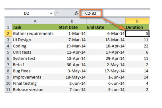
1. First, enter your project data in an Excel spreadsheet. List every task in a separate row. Enter the Start date, End date, and Duration to structure your project plan. Only the Duration and Start date are necessary for the Gantt chart.
   
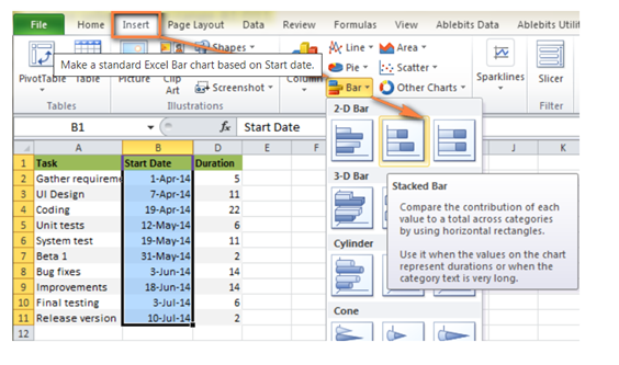
2. Set up the usual Stacked Bart chart in Excel. Select your Start Dates with column header, then click “Insert”. Open Charts group and select “Bar”. From the 2-D bar section, select "Stacked Bar".
   
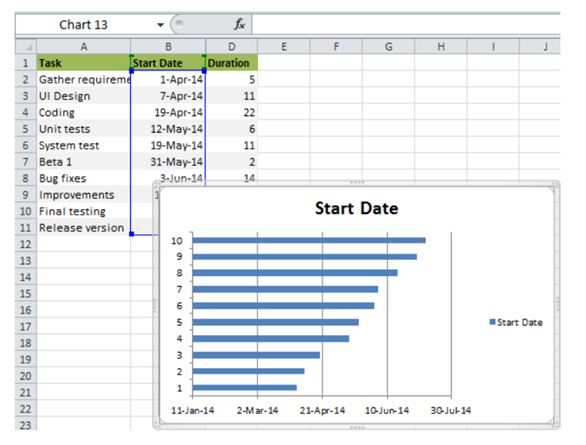
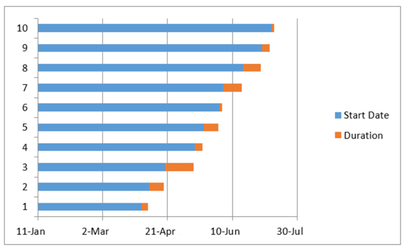
3. You will have the Stacked bar added to your spreadsheet as a result.
   
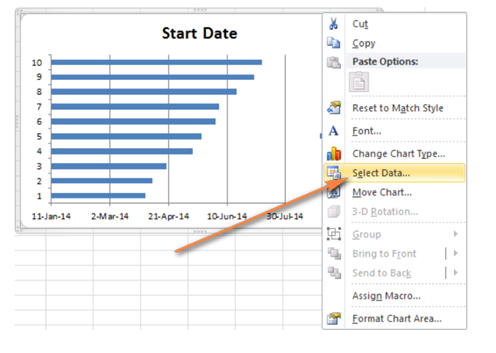
4. Click right in the chart and a context menu will appear. Choose “Select Data”.
   
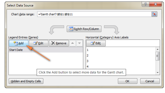
5. From the Select Data Source window, click “Add” to add Duration in your Gantt Chart.
   
6. Edit Series window will open and type “Duration” in the Series name field.
   
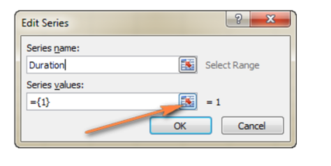
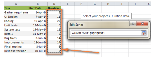
7. Click on the icon next to the Series values field and a small Edit Series window will open. Select your project Duration.
   
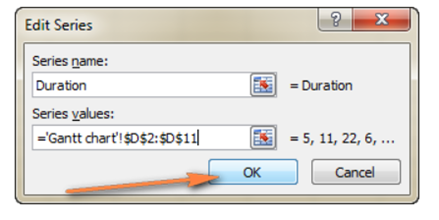
8. Click the Collapse Dialog icon and it will bring you back to the previous Edit Series. Click “Ok”
   
9. Now both Start Date and Duration are added in the Select Data Source window.
   
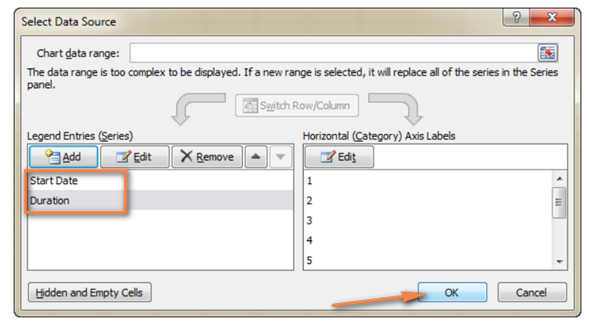
10. Click “Ok” and see the resulting bar chart.
    
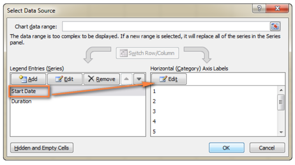
11. Now for adding task descriptions to your Gantt chart, again open the Select Data Source window. Click “Edit” on the right panel.
    
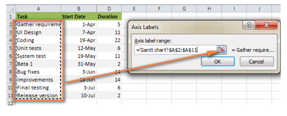
12. Axis Label window will open. Then select your tasks and add them the same way as Durations. Don’t include the column header. Then double click “Ok”.
    
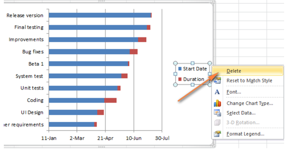
13. Right-click and select “Delete” to remove the chart labels block.
    
14. Now task descriptions are on the left side of your Gantt chart.
    
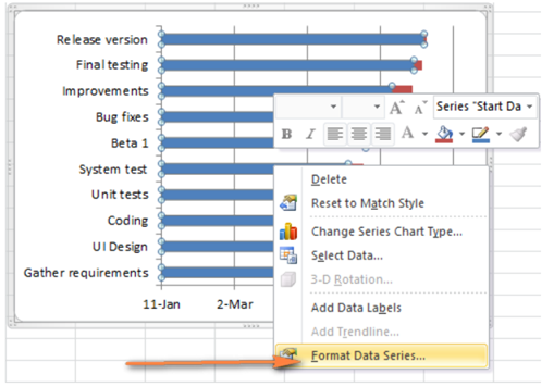
15. Now you have to transform the Bar graph into the Excel Gantt chart. Select all the blue bar in your Gantt chart and right-click. Then select “Format Data Series”.
    
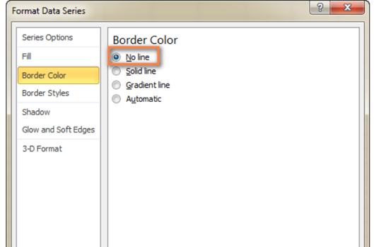
16. Format Data Series window will open and click on the “Fill” tab and select “No Fill”.  Then choose “No line”  from the “Border Color” tab. 
    
17. Now see your tasks are listed in reverse order, so we have to fix this. Click on the tasks and this will open “Format Axis”. Click “Axis Options”. Choose “Categories in Reverse Order.
18. So now your tasks are properly arranged and your Gantt chart is almost ready.
19. You can do some more edits and make your chart look like an ideal Gantt chart.
    
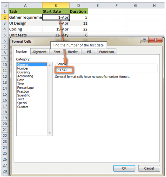
20. You can bring your tasks a little closer to the left vertical axis by removing the space. Right-click on the first Start date and select “Format Cells”, then “General”. Write the number that appeared.
    
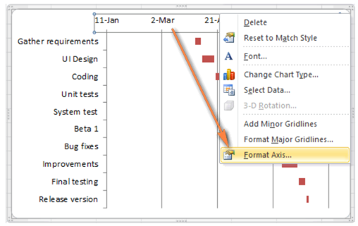
21. Then select all the dates and right-click to open the context menu. Select “Format Axis”
    
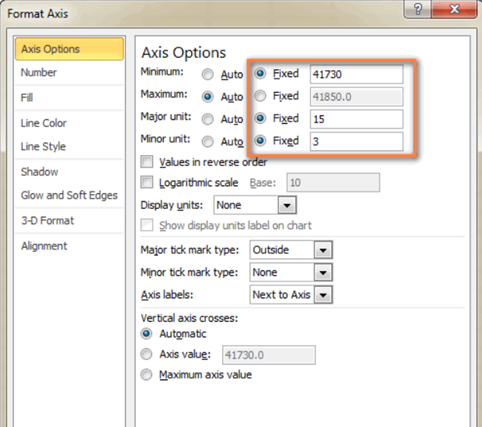
22. In the “Axis” option change “Minimum” to “Fixed” and type the previous number you wrote. Select “Fixed” for “Major unit”. Also, choose “Fixed” for “Minor unit”. Then add suitable numbers you want for the date intervals.
    
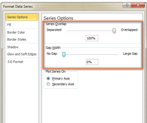
23. Select all the orange bars and right-click to open “Format Data Series”. Apply 100 percent in "Separated" and 0 percent in "Gap Width".
    
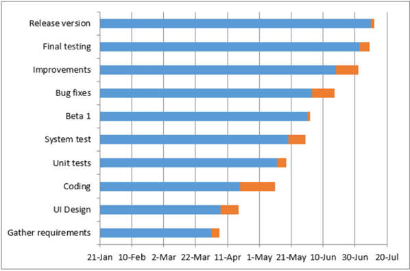
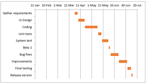
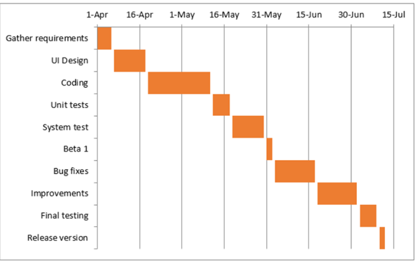
24. Finally, your Gantt Chart is ready in Excel.
    

So, following these, you can easily make a simple and nice-looking Gantt Chart in Microsoft Excel. 

Summary: How to use excel template to produce a Gantt Chart?

• Go to the 'File' option and select the 'New' option.
• There is a search bar where you can type in 'Gantt Chart' or 'Project Planner'.
• Choose the template called 'Use this template', which should be one of the first ones.
• Once you are on the new worksheet, you can start adding in tasks and milestones.
• Tasks and milestones should be listed in the first column. Click on cell B2 and change the text to what your first task is.
• In cell B3, click the small arrow to bring up the dialog box that says 'Fill Series'. Click on this and it will fill in a list of dates automatically so that you can have a timeline made for you.
• In cell C2, you can type what your second task is. You can continue this process down as far as needed.
• Once all of your tasks are added, you can change the title to reflect what your project is called. Then, when you are ready, print out your Gantt chart.
• The steps outlined above will help make it easier to use a Gantt.